Find Stationary Distribution of Markov Chain using Stochastic Simulation (Gillespie's) in Python

This is the ad hoc tutorial on how to simulate continuous Markov Chain using Gillespie’s Direct Stochastic Simulation algorithm and find its stationary distribution and estimate the accuracy.

Below content is complementary to the video tutorial above.

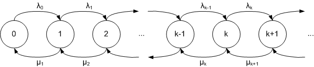
We will use a birth and death process with a \(M/M/1\) queue which is simple Markov model, where \(\lambda_i = \lambda\) is arrival (birth) rate, \(\mu_i = \mu\) is service (death) rate. The load of the system is \(\rho=\lambda / \mu \lt 1\). The state of the system \(n\) is the number of customers in the system. \(p(n)= (1-ρ) \rho^n\) is the stationary distribution of the state \(n\). We will compare \(p(n)\) with the result of the stochastic simulation using Mean Squared Error (MSE).

Gillespie’s Direct method

Gillespie’s Direct method is variation of Monte Carlo simulation. Below is the algorithm description:
Transition rate from the state x to state i is denoted by \(q(x,i)\).

Define total simulation time \(T\) and set current time \(t = 0\);
Initialize the state of the system \(x\) – choose randomly or set zero state;
Find the sum \(Q\) of all the possible transition rates from the current state \(x\);
Simulate the time \(\Delta t\) until the next transition by drawing from an exponential distribution
with parameter Q;
Generate a random number \(r\) from a uniform distribution;
Set the next state \(n\) as follows:
if \(0 \lt r \lt q(x,0)/Q\) set \(x = 0\),
else if \(q(x,0)/Q \lt r \lt (q(x,0)+q(x,1))/Q\) set \(x = 1\),
else if \(\sum \limits_{i=0}^{n-1}(q(x,i))/Q \lt r \lt \sum \limits_{i=0}^{n}(q(x,i))/Q\) set \(x = n\),
Update the current time: \(t = \Delta t+t\);
Repeat 3-7 until \(t \le T\).

Python source code

Github: https://github.com/mamedshahmaliyev/adhoctuts/blob/master/python/math/mc_gillespie.py

'''Stochastic simulation of birth and death process with a Markov M/M/1 queue using Gillespie Direct method'''
import random
def getSystemParameters():
return {'lambda': 5, 'mu': 10}
def nextStateSpace(currentState):
'''All the possible transition rates from the currentState: dict(possibleState: rate)'''
p = getSystemParameters()
nextStateSpace = {currentState + 1: p['lambda']}
if currentState > 0: nextStateSpace[currentState - 1] = p['mu']
return nextStateSpace
def simulate(initialState = 0, simulationTime = 5000):
currentState = initialState
timePassed = 0
reachedStates = {} #dict(state:sojournTime); sojournTime is total spent time for the state
nextStatesAll = {} #dict(state:nextStates);
while timePassed < simulationTime:
if currentState not in reachedStates: reachedStates[currentState] = 0
if currentState not in nextStatesAll: nextStatesAll[currentState] = nextStateSpace(currentState)
nextStates = nextStatesAll[currentState]
transRateSum = sum(nextStates.values())
nextInterval = random.expovariate(transRateSum)
r = random.uniform(0,1)
prevRateSum = 0
for state in nextStates:
if r > prevRateSum / transRateSum and r < (prevRateSum + nextStates[state]) / transRateSum:
reachedStates[currentState] += nextInterval
currentState = state
break
prevRateSum += nextStates[state]
timePassed += nextInterval
totalTime = sum(reachedStates.values())
return {state: reachedStates[state] / totalTime for state in reachedStates}
def exactStationaryDistribution(state):
p = getSystemParameters()
systemLoad = p['lambda'] / p['mu']
return (1 - systemLoad) * systemLoad ** state
#----------------------- Run the experiment ----------------------------#
sd = simulate(0, 10000)
mse = 0 # mean squared error
for state in sd:
e = exactStationaryDistribution(state) # exact distribution
mse += (sd[state] - e)**2
print('[ State -',state,'] [ Simulation -', "{:.7f}".format(sd[state]),'] [ Exact -',"{:.7f}".format(e),' ]')

print ("Mean Squared Error (MSE):", "{:.7f}".format(mse / len(sd)))

#----------------------- Visualize the accuracy based on Simulation Time ----------------------------#
serie = {'x':[],'y':[]}
for t in [500,1000,2000,3000,5000,7000,10000,15000,20000]:
mse = 0
sd = simulate(0, t)
for state in sd:
e = exactStationaryDistribution(state) # exact distribution
mse += (sd[state] - e)**2
serie['x'].append(t)
serie['y'].append(mse / len(sd))

import matplotlib.pyplot as plt
fig = plt.figure(1,figsize=(7.5, 3.9), dpi=80)
plt.plot(serie['x'], serie['y'], label='MSE Dependence on Simulation Time')
ax = plt.gca();
ax.set_xlabel('Simulation Time')
ax.set_ylabel('MSE')
plt.grid(color='#A9A9A9', linestyle='--', linewidth=0.5)
plt.show()

Above code could be applied to simulate any Markov model. To use the above code for another model you should update getSystemParameters and nextStateSpace functions correspondingly and use simulate function to simulate the model and find stationary distribution.

The accuracy estimation – MSE (Mean Squared Error) dependence on the Simulation Time

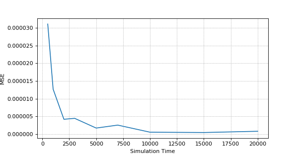
The above is sample result and it may differ on your experiment, but general picture should be the same.

Related resources: